Fine-Tuning a Semantic Segmentation Model on a Custom Dataset and Usage via the Inference API

Authored by: Sergio Paniego

In this notebook, we will walk through the process of fine-tuning a semantic segmentation model on a custom dataset. The model we'll be using is the pretrained Segformer, a powerful and flexible transformer-based architecture for segmentation tasks.

For our dataset, we'll use segments/sidewalk-semantic, which contains labeled images of sidewalks, making it ideal for applications in urban environments.

Example use-case: This model could be deployed in a delivery robot that autonomously navigates sidewalks to deliver pizza right to your door 🍕

Once we've fine-tuned the model, we'll demonstrate how to deploy it using the Serverless Inference API, making it accessible via a simple API endpoint.

1. Install Dependencies

To begin, we’ll install the essential libraries required for fine-tuning our semantic segmentation model.

2. Loading the Dataset 📁

We'll be using the sidewalk-semantic dataset, which consists of images of sidewalks collected in Belgium during the summer of 2021.

The dataset includes:

• 1,000 images along with their corresponding semantic segmentation masks 🖼
• 34 distinct categories 📦

Since this dataset is gated, you'll need to log in and accept the license to gain access. We also require authentication to upload the fine-tuned model to the Hub after training.

Review the internal structure to get familiar with it!

Since the dataset only includes a training split, we will manually divide it into training and test sets. We'll allocate 80% of the data for training and reserve the remaining 20% for evaluation and testing. ➗

Let's examine the types of objects present in an example. We can see that pixels_values holds the RGB image, while label contains the ground truth mask. The mask is a single-channel image where each pixel represents the category of the corresponding pixel in the RGB image.

3. Visualizing Examples! 👀

Now that we’ve loaded the dataset, let’s visualize a few examples along with their masks to understand its structure better.

The dataset includes a JSON file containing the id2label mapping. We’ll open this file to read the category labels associated with each ID.

Let's assign colors to each category 🎨. This will help us visualize the segmentation results more effectively and make it easier to interpret the different categories in our images.

We can visualize some examples from the dataset, including the RGB image, the corresponding mask, and an overlay of the mask on the image. This will help us better understand the dataset and how the masks correspond to the images. 📸

4. Visualize Class Occurrences 📊

To gain deeper insights into the dataset, let’s plot the occurrences of each class. This will allow us to understand the distribution of classes and identify any potential biases or imbalances in the dataset.

5. Initialize Image Processor and Add Data Augmentation with Albumentations 📸

We will start by initializing the image processor and then apply data augmentation 🪄 using Albumentations. This will help enhance our dataset and improve the performance of our semantic segmentation model.

6. Initialize Model from Checkpoint

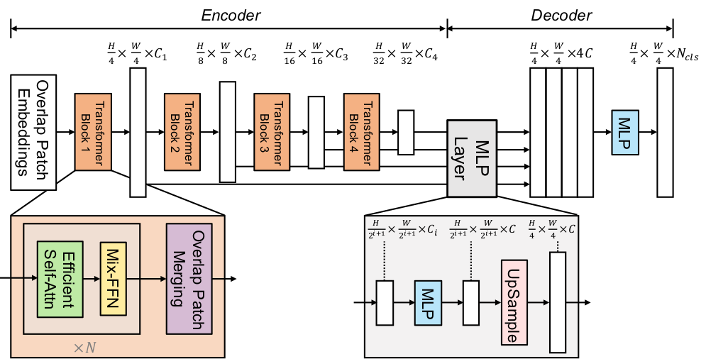
We will use a pretrained Segformer model from the checkpoint: nvidia/mit-b0. This architecture is detailed in the paper SegFormer: Simple and Efficient Design for Semantic Segmentation with Transformers and has been trained on ImageNet-1k.

7. Set Training Arguments and Connect to Weights & Biases 📉

Next, we'll configure the training arguments and connect to Weights & Biases (W&B). W&B will assist us in tracking experiments, visualizing metrics, and managing the model training workflow, providing valuable insights throughout the process.

8. Set Custom compute_metrics Method for Enhanced Logging with evaluate

We will use the mean Intersection over Union (mean IoU) as the primary metric to evaluate the model’s performance. This will allow us to track performance across each category in detail.

Additionally, we’ll adjust the logging level of the evaluation module to minimize warnings in the output. If a category is not detected in an image, you might see warnings like the following:

RuntimeWarning: invalid value encountered in divide iou = total_area_intersect / total_area_union

You can skip this cell if you prefer to see these warnings and proceed to the next step.

9. Train the Model on Our Dataset 🏋

Now it's time to train the model on our custom dataset. We’ll use the prepared training arguments and the connected Weights & Biases integration to monitor the training process and make adjustments as needed. Let’s start the training and watch the model improve its performance!

10. Evaluate Model Performance on New Images 📸

After training, we’ll assess the model’s performance on new images. We’ll use a test image and leverage a pipeline to evaluate how well the model performs on unseen data.

The model has generated some masks, so we can visualize them to evaluate and understand its performance. This will help us see how well the model is segmenting the images and identify any areas for improvement.

11. Evaluate Performance on the Test Set 📊

12. Access the Model Using the Inference API and Visualize Results 🔌

Hugging Face 🤗 provides a Serverless Inference API that allows you to test models directly via API endpoints for free. For detailed guidance on using this API, check out this cookbook.

We will use this API to explore its functionality and see how it can be leveraged for testing our model.

IMPORTANT

Before using the Serverless Inference API, you need to set the model task by creating a model card. When creating the model card for your fine-tuned model, ensure that you specify the task appropriately.

Once the model task is set up, we can download an image and use the InferenceClient to test the model. This client will allow us to send the image to the model through the API and retrieve the results for evaluation.

We will use the image_segmentation method from the InferenceClient. This method takes the model and an image as inputs and returns the predicted masks. This will allow us to test how well the model performs on new images.

With the predicted masks, we can display the results.

It’s also possible to use the Inference API with JavaScript. Here’s an example of how you can consume the API using JavaScript:

import { HfInference } from "@huggingface/inference";

const inference = new HfInference(HF_TOKEN);
await inference.imageSegmentation({
    data: await (await fetch("https://picsum.photos/300/300")).blob(),
    model: "sergiopaniego/segformer-b0-segments-sidewalk-finetuned",
});

Extra Points

You can also deploy the fine-tuned model using a Hugging Face Space. For example, I have created a custom Space to showcase this: Semantic Segmentation with SegFormer Fine-Tuned on Segments/Sidewalk.

Conclusion

In this guide, we successfully fine-tuned a semantic segmentation model on a custom dataset and utilized the Serverless Inference API to test it. This demonstrates how easily you can integrate the model into various applications and leverage Hugging Face tools for deployment.

I hope this guide provides you with the tools and knowledge to confidently fine-tune and deploy your own models! 🚀